Research Instruments

Numbers Click here
Law of Comparative Judgement Click here
Scenic Beauty Estimation Click here
Rating of photographs Click here
Paired photographs Click here
Q-sort of photographs Click here
Visitor employed photographs Click here
Semantic differential Click here
Adjective checklist Click here
Physiological tests Click here
Interviews and questionnaires Click here
Measurement of features in photographs Click here
Research instruments – conclusions Click here

The basic methodological approach involves measuring the relationship between the landscape as perceived by human observers stating their preferences for the landscape, usually by use of some rating scale (e.g. 1 – 10) or by other physiological and psychological measures. The landscape is known as the independent variable because it remains constant and invariable regardless of who views it, rates it, measures it or examines it. Human observers, on the other hand, are not constant but their preferences and reactions to a landscape can vary widely influenced by a range of personal, interpersonal, cultural and other factors. Figure 1 summarizes the three elements of the method.

Most of the research instruments are used to evaluate the dependent variables, measuring the preferences of observers and how they vary with the quality of the landscape. This is achieved through statistical measures, including correlation, multiple regression and factor analysis. Other studies which compare the preferences of one population sample with another use no independent variable.

Numbers

In measuring anything, including landscape quality, numbers are used. However, numbers come in a variety of capabilities – according to Stevens (1946) there are four types of numbers:

Nominal, the weakest form, merely take the form of labels or categories, such as the numbers on the backs of football players for identification. Numbers can be used for classes, e.g. males = 1, females = 2. Such classes or numbers have no order (i.e. they are random) and have no sense of relativity (i.e. none is better than the other).

Ordinal implies a relative ranking, e.g. one mineral is harder than another, an odour is more pleasant than another, this landscape is more appealing than that one. While relativity is apparent, the intervals between classes are not necessarily equal, nor is there a baseline – i.e. zero point.

Interval measures are quantitative in the usual sense of the word. It provides a ranking between classes and an equal spacing between them, however, a zero point is arbitrarily assigned. The temperature scale is an interval scale – the units are of equal size and the zero on the Celsius scale is based on the freezing point of water; it does not denote the absence of temperature in the way that 0^° Kelvin does (i.e. absolute zero). An interval scale enables precision about the differences in magnitude of objects; one can state that one is twice that of the other. Interval scales are commonly used in psychology. 

Ratio measures are the strongest form of numbers. They are sometimes known as cardinal numbers. Relativity between objects is defined, the intervals between units are equal, and an absolute zero point is included, which means the complete absence of the characteristic being measured. Ratio measures have all the properties of interval measures plus an absolute basepoint. Measures of weight and distance are examples.

The four qualities of numbers are summarized in Table 1.

Table 1 Summary of Types of Measures

Most landscape research assumes that the data is interval whereas in fact they are mostly ordinal. According to Schroeder (1984), “The simplest scaling methods treat the non-interval scale problem by ignoring it, they assume that rating data already possess interval properties and analyze them accordingly.”

A range of research instruments for measuring landscape preferences have been developed, ranging from simple to the sophisticated.

The sophisticated research methods produce interval-type data and these include the Law of Comparative Judgement (LCJ) method and the Scenic Beauty Estimation (SBE) method, developed from psychophysics.

Psychophysics originated in the 19^th century through the work of a German physicist, Gustav Fechner (1801 – 87), who defined it as “an exact science of the functional relations of dependency between body and mind” (Torgenson, 1958), or the measurement of sensations and perception (Lindzey et al, 1988) – in other words, it measures how the brain interprets information provided by the senses (see Visual perception).

A basic assumption of psychophysics is that people are reasonably consistent in making judgements or choices among options. In regard to landscapes, people are unlikely to switch their preferences markedly during a test. Although some variability is acknowledged, it is assumed to display a normal distribution with the true value being represented by the mean (Hull et al, 1984).

According to the Macaulay Institute (2013):

Of all landscape assessments, (psychophysical) methods have been subjected to the most rigorous and extensive evaluation. They have been shown to be very sensitive to subtle landscape variations and psychophysical functions have proven very robust to changes in landscapes and in observers. Relying on ordinal or interval scales of measurement, psychophysical methods have consistently been able to provide different landscape-quality assessments for landscapes that vary only subtly.

Law of Comparative Judgement

During the 1920s, Louis Thurstone (1887 – 1955) developed psychophysical scaling laws that enabled the accurate measurement of those psychological attributes resulting from stimuli but which had no physical manifestation. His Law of Comparative Judgement (Thurstone, 1927) is one of the key foundations for research into landscape quality and has been used widely across a range of disciplines, including psychology, engineering, marketing, and ergonomics (Hull, 1986).

The problem that Thurstone addressed was that individuals making judgements about the same feature would give similar but not identical responses at different times. Furthermore, while some individuals are consistent in their reliability, others may be very inconsistent. If respondents use, say, a 10-point scale and are asked to rate some feature, they may regard the interval differences between 5 and 6 as different than between 8 and 9. Thus, while the researcher may treat each unit as equal, the respondents may not. Scaling methods provide a means of transforming the raw responses into accurate and reliable scale values that reflect the perceived properties of the features.

Thurstone defined five cases in the Law of Comparative Judgement (LCJ), but we will concern ourselves only with the third case which involves several observers, each judging each pair of scenes several times. This is widely used in landscape research with photographs of scenes providing the stimuli and assuming that each photograph may be judged independently of others. Two photographs are shown side by side. The observer judges between the two and chooses one based on whatever criterion is defined – such as the preference of one over the other. Each photograph is compared successively with every other photograph. No single photograph appears twice in succession, and the aim should be to space them as far apart as possible. No two photos should be judged equal.

A limitation of the method is that the number of paired comparisons grows rapidly with the number of photographs. With n stimuli, there are n(n-1)/2 pairs of stimuli required. It is generally impractical to go beyond about 15 pairs (Guildford, 1954). This would require 105 paired comparisons, which are about as many as one could reasonably expect a survey participant to undertake. Increasing the number of photographs by one (to 16) increases the paired comparisons to 120, a sizeable increase for only one extra photograph. An experiment requiring observers to make 120 comparative judgements could suffer from observer fatigue (Hull et al, 1984). While most of the studies using the LCJ method had less than 15 pairs of photographs, one used 29 pairs, requiring 406 paired comparisons (Whitemore et al, 1995). Figure 2 indicates the number of paired comparisons that need to be made for n photographs. Thus for 20 scenes, 190 paired comparisons must be made.

The LCJ method requires a large number of comparisons of each stimulus to provide sufficient data for analysis, so a balance has to be struck between exceeding the patience of the observers and providing sufficient data for analysis.

Through a series of mathematical steps and data transformations, the LCJ method provides interval scaling between preferences. This enables the results to be analyzed using standard statistical methods. A key researcher who has used the LCJ method extensively is Greg Buhyoff, who has used the method in twelve of his studies.

Scenic Beauty Estimation

The second psychophysical method is the Scenic Beauty Estimation (SBE) method that was developed in the mid-1970s by Terry Daniel, a psychologist at the University of Arizona, and Ron Boster, a forester with the US Forest Service. The SBE method transforms ordinal ratings to an interval scale SBEs.

SBE method has its origins in both the Law of Categorical Judgement and the Theory of Signal Detection. The Theory of Signal Detection has close parallels with Thurstone’s law (Green & Swets, 1966) and grew out of research to detect a weak message over a noisy telephone (Lindzey et al, 1988). The theory is based on the research finding that the cognitive state of the person doing the detecting, their biases and expectations, influences the results they attain. Providing rewards or punishments for the detection changes the cognitive state and one’s willingness to make false alarms or misses. However, one’s true sensitivity remains the same. Signal Detection Theory allows the researcher to separate spurious and real influences so as to determine the observer’s true sensitivity, provided the observer is neither cautious nor reckless.

Applying SBE to landscapes, an observer may form a negative judgement about Landscape A that they do not like it. Landscape B, however, exceeds the implicit criterion the observer sets and results in a positive judgement – “I like it”. If, however, the observer’s standards were raised for some reason, their judgement:

“would be negative for both landscapes, even though their perceived beauty has not changed. Thus, scenic beauty judgements depend jointly on the perceived properties of the landscape and the judgemental criteria of the observer” (Daniel & Boster, 1976, the author’s emphasis).

Ideally, if each observer rated a landscape out of a possible top score of 10, a rating of, say, 7 would be the equivalent across observers. However, this would be unusual because each observer’s criterion is unique, and the same landscape will be rated differently by different observers, making the scoring difficult to interpret. For example, one observer may rate a landscape as 3 out of 10, applying a very high aesthetic criterion, while another having a low aesthetic standard may score it as 8.

These and other problems of observer differences are solved through the SBE method, in which a measure of landscape beauty “independent of observer judgemental criteria” is derived.

The SBE method involves three stages: 1. taking color photographs of the landscape, 2. presenting these to participants for evaluation and 3. evaluating their judgements. Daniel & Boster developed the method in ponderosa forest on flat topography, but it has been used across many landscapes.

Like the LCJ method, the SBE method assumes that all individuals will categorize each slide in essentially the same location on their respective scenic beauty continuum, and that differences among individuals are normally distributed. These categories can then represent a basis from which measurements of scenic beauty can be made. Each category is indicated by a distribution, reflecting both individual differences and variability in perceptual and judgemental processes. The mean of the distribution is assumed to represent the true category.

Hypothetical results of a survey are presented in Figure 3. The three graphs indicate the scenic beauty scales assigned the average ratings given by the three observers to each of the landscapes are as follows:

Table 2   Derivation of Scenic Beauty Estimation (SBE) for Three Scenes

Brown & Daniel (1990) Note: Stimuli 1, 2, 3 are individual scenes and indicates the scores by three observers on the scale 1 – 10. cf = cumulative frequencies, cp = cumulative probabilities and Z is Standard Normal Distribution (Z tables).

While the order of these is the same, the scores given for each landscape differ between observers even though the perceived scenic beauty values are identical for all observers. Table 1 summarizes the derivation of the SBE score using the “by slide” or “by stimulus” method of Daniel & Boster. This method uses multiple observers to rate the scenes and from this, a distribution of ratings for each scene is obtained. The rating distributions are converted to frequencies for each rating category (e.g. 1 – 10) and Z values derived. Daniel and Boster’s alternative method is “by observer,” which uses few observers rating multiple scenes of a given landscape.

Daniel & Boster used the SBE method in relation to forest management and applications included deriving aesthetic contour maps for National Forest areas, examining the effects of timber harvesting on scenic beauty, and identifying the factors that affect the SBE scores. The amount and distribution of felled timber and stumps had a negative effect, while tree density, tree diameter and crown-canopy cover each contributed positively. It has also been used to estimate the scenic effect of beetle damage on trees, the forest factors that contribute to scenic beauty, the changes to scenic beauty over time with forest maturation, tradeoffs between scenic beauty and timber value, effect of distance on scenic beauty, cultural differences in scenic beauty estimates, effect of scene composition on scenic beauty estimates, and alternative options for the landscape and their impact on scenic beauty.

Because the LCJ and SBE methods both produce interval scale metrics, they do not define absolute scenic values (i.e. no benchmark zero point is available), only relative differences. Thus, the scores derived from different studies of different landscapes cannot be compared as a SBE score of say 60 in one area bears no relation to the same score in another area. However, Hull considers it possible to compare two sets of landscapes that share some scenes (Hull, 1987).

From a user’s viewpoint, it is difficult to convey what a landscape with an SBE of -28 is compared with a second landscape of -7 and a third of +35. Using a 1 – 10 rating scale they can be described as 5, 6 and 8, which communicates far more clearly their relative quality. Used carefully, this scale also enables comparisons of landscapes from different surveys.

While there may be some appeal in the sophistication of the LCJ and SBE methods, it has been suggested that these complex methods do not produce any real gain over simpler methods. Schroeder (1984) tested both complex and simple methods for rating landscape quality and concluded that there was no discernible difference – “even the most sophisticated of scaling methods seems to produce results that are equivalent to a simple mean rating.”  He commented that rating scales that are “often maligned as ‘merely ordinal’, may actually approximate interval scale data more closely than many people suspect.” Thus a simple rating scale, such as 1 (low) to 10 (high) as used by the author suffices. Such scales are far more intuitively acceptable than the negative to positive integers that result from the SBE method.

Schroeder also makes the point in view of his research that small samples may be adequate as they produce acceptable intergroup reliability. Typically, researchers have a rule-of-thumb of 15 – 25 raters whereas Schroeder considers that 9 to 15 would be adequate. Prior to Internet-based surveys, the cost of the survey largely related to the number in the sample so this was a significant consideration but is less so now.

The following are research instruments that are generally simpler to use than the LCJ and SBE.

Rating of Photographs

Rating of photographs is the single most prevalent method, and its attraction lies in its simplicity and effectiveness. Typically, photographs are presented as prints, as slides, or more commonly now, digital images are presented on a computer screen via the Internet, and respondents rate each scene. The advantage of the Internet is that randomization can be built into the order so that each viewer sees them in a different order. This overcomes issue of a rating of a scene being influenced by the previous scene. It also offsets the problem of fatigue affecting the ratings as the survey can be delayed for a period. Surveys should commence with a few scenes to “prime” the viewer of the range of images to be presented from low to high quality, thereby cueing their brain regarding their rating.

Online survey companies such as Survey Monkey are available with easy-to-use tools to construct the survey, input the images, and collect and even analyze the results. Other instruments include: Question Pro, eSurvey Pro, Zoomerang, Survey Gizmo, Free online survey, Fluid surveys, Qualtrics, Survey Expression, Goodle Consumer Surveys, and Smart-Survey. According to Roth (2006), the “scenic quality categories of visual variety, beauty, visual naturalness as well as overall scenic quality can be validly recorded on the Internet.”

Rating scales vary among studies. Some use an odd number, say 1 – 9 so that the mid-point is an integer (5) whereas for the 1 – 10 scale the mid-point is 5.5. Some surveys use a 5 or 7 points. However, the scale needs to provide sufficient discrimination between scenes and scales of 5 and possibly 7 points fail in this. On the other hand, a 1 – 100 scale provides too much discrimination, and it can be difficult for a viewer to discriminate say between 65 and 66. The scale should not include the zero, 0, as there is logically no scene of zero rating. Even scenes of a flat plain without any land form, land cover, land use, water or any other feature have been found to rate 3 – 4 on a 1 – 10 scale.

The author’s experience is that the 1 – 10 scale works very well; it provides sufficient discrimination and is most easily used by viewers. Most scales go from worst (1) to best (10) as the reverse (best 1 – worst 10), can be confusing for participants and they can revert to the worst-best scenario after a few scenes, which makes data analysis problematic.

Rating scales are used in landscape surveys to rate the aesthetic quality of the landscape as well as many other attributes, including Kaplan’s variables of coherence, complexity, legibility and mystery; tranquillity, naturalness and familiarity. The author’s surveys also assess the visual significance of components in the scenes, including land form, vegetation, land uses, water, diversity and naturalness. These components are rated on a 1 – 5 scale.

The number of photographs used in studies varies from 6 to 180 with the majority in the 40 – 60 range. However, with Internet surveys, longer surveys can be used as the person can pause the survey when fatigued and return to it later.  Table 3 indicates the average time taken to complete four of the author’s surveys. In the early days of the Internet, many respondents used dial-up connections but there was little difference in their times compared with broadband. Figure 4 shows the duration for several surveys.

Table 3 Effect of Internet connections on survey times

While rating of scenes enables comparisons of their ratings from a common base, rankings only provide an ordinal hierarchy of scenes, which is difficult to analyze.

Paired Photographs

A group of photographs are allocated into pairs and the preference for each photograph in each pair is recorded. This differs from the LCJ method in that each photograph is different, so the sample is not limited to a relatively small number of photographs. Studies have used up to 120 photographs in 60 pairs. The method is particularly popular in Spain – 11 out of the 16 studies using this method were undertaken in Spain by researchers including Abello, Bernaldez, De Lucio, Marcia and Rodenas.

Q-Sort of Photographs

The Q-sort procedure was originally developed for personality assessment (the ‘Q’ prefix has no special significance). Based on psychological research, which indicates that the human senses are not capable of discriminating sensory perceptions into more than nine categories (Pitt & Zube, 1979), participants are asked to sort a set of photographs into five or seven piles. Even numbers of piles are avoided so as to permit a central group.

The Q-sort allows a large number of stimuli to be evaluated. An advantage it has over a rating form is that the participant can shift items back and forth as they proceed (Cronbach, 1970). Thus, the photographs in a given pile at the end of the sorting can be regarded as approximately equivalent. Forcing the participant to allocate a pre-set number of photographs to each pile is regarded as being preferable to an unforced choice. Swaffield and Fairweather in New Zealand have used Q sort in several studies.

Visitor Employed Photographs (Participant Photography)

As the name suggests, this technique uses the selection of photographs taken by visitors as an indicator of landscape preferences. The method involves loaning park visitors an inexpensive and easily operated film camera, and asking them to take photographs of given subjects. This may be as broad as “anything they wish” (Cherem & Driver, 1983), preferred scenes, anything of interest, or may be used to provide material for use in framing a questionnaire (Hammitt, 1979).

Gabriel Cherem developed the method in the early 1970s as a means of eliciting the public’s view of aesthetic objects. Cherem & Driver (1983) evaluated the method in landscape research, trialling it in three studies. They provided cameras to hikers on a trail (of 512 cameras loaned, only 6 were not returned) and from the hundreds of photographs taken, identified ‘consensus photographs’ (i.e. scenes photographed by 10% or more of the participants). They acknowledge that the 10% figure is arbitrary and could be set higher or lower, but it serves to provide a “concrete representation of a scene which offers some common degree of perceptual interest.”

Hull & Revell (1989) used the participant photography method in a study in Bali of cross-cultural landscape preferences among the Balinese and Western tourists. Based on the photographs taken, consensus scenes were identified based on 10% of the responses from each culture.

In an evaluation of the method, Chenoweth (1984) concluded that it is a tool that “deserves serious consideration along with other tools for understanding people’s reaction to the landscape …”

Semantic Differential

The semantic differential (SD) is the first of the descriptive methods used in landscape research. Charles Osgood developed the SD technique in the mid-1950s as an objective method of measuring perception, meaning and attitudes. It has been used for assessing the reactions of observers to different types of environmental stimuli, including the architecture of buildings; rooms and interiors; snow, rain, fog and other meteorological phenomena; beach scenes; and roadside scenery.

The SD technique is based on the following prerequisites (Osgood & Suci, 1955):

• Judgement can be made in terms of a continuum, definable by polar terms (i.e. opposites such as like – dislike);
• The many different ways in which meanings can vary can be represented by a single dimension (e.g. scenic quality as a term covering a landscape’s aesthetic qualities);
• A limited number of continua can be used to define a quality within which the meaning can be specified.

The SD technique involves participants scoring photographs on a series of bipolar semantic scales, each of which has, say, a 7-point gauge. The scales might be expressed in terms of: common/ unusual, pleasant/untidy, obvious/mysterious, artificial/natural, weak/powerful and barren/fertile.

The SD technique is a mature methodology that has been used extensively in landscape preference assessment.

Adjective Checklist

The second descriptive method is the adjective checklist that has been used for the evaluation of landscapes. In 1972, Kenneth Craik developed a Landscape Adjective Check List (LACL) based on descriptions of 50 natural landscape scenes by students. He asked students to list 10 adjective descriptors of each scene and while not all were able to achieve this, adjectives that were used six or more times comprised a list of 1196 distinct items. The LACL comprised 240 adjectives. He proposed that the list be used to:

• derive impressions of landscapes quickly from large samples in the field
• statistically compared descriptions of the same landscapes
• record impressions of landscape
• assess change in landscapes
• evaluate the effectiveness of photographs, sketches and other surrogates of landscapes

Craik (1975) used the list in a field assessment of landscape in Marin County, California and identified 104 adjectives that were used by 10% or more of the participants. It identified the following attributes of the area: clean, hilly, tree-studded, grassy, pleasant, beautiful, natural, green, peaceful, and sunny. Factor analysis was then used to identify four descriptive landscape factors: serene/gentle, dry/barren, beautiful/ picturesque, and blooming/cultivated.

Kane (1976, 1981) in a study of South Australian landscape for the National Trust, developed and applied a bipolar list of 21 adjectives, of which 14 were significant to South Australians as descriptive of their landscape. The adjective pairs included wet/dry, cold/warm, private/public, unstimulating/stimulating, and disordered/order. Responses were transformed into a landscape rating score through application of a weighting factor derived from an earlier evaluation of 40 adjective pairs, and a selection of those which related most to beautiful/ugly and like/dislike. The scoring of adjective pairs was undertaken by ten respondents and applied to 46 scenes throughout South Australia. Checklist scores ranged from a high of 80 down to 29.

The adjective checklist method has not been widely used but can provide an effective and quick method of assessing impressions of a landscape.

Physiological tests   

While psychophysical tests and other preference rating methods assume that human cognitive and affective responses to landscapes can be expressed and measured, physiological tests aim to measure these responses more directly. Physiological effects are autonomic (i.e. self-governing) responses of the human body to environmental stimuli – the subject cannot intentionally create them.

Roger Urlich who has postulated a landscape theory based on its affective effects has carried out a range of studies using physiological tests. In Ulrich, 1981, he used alpha wave amplitude and heart rate to compare reactions to photographs of scenes of natural and urban environments. In Urlich et al, 1991, he used a battery of tests: electrocardiogram, pulse transit time (correlates with systolic blood pressure), spontaneous skin conductance responding, and frontalis muscle tension – to assess the rate of recovery from stress from a stressful movie during exposure to videos of natural and urban scenes. There have been many other studies by researchers using physiological tests.

Physiological tests are complex and require specialist equipment and expertise in their administration.

Interviews and Questionnaires

Interviews and questionnaires play an important role in landscape research and are often used in association with other methods. About 50% are field administered surveys. They require a large number of respondents and therefore, are expensive in cost and resources required – one survey of 242 averaged only 4 interviews a day – 60 days total.

Measurement of features in photographs

The final method examined is the only one that provides an objective measure of the composition of landscapes as depicted in photographs. It is therefore, the only measure that has been developed of the independent variable (i.e. the landscape).

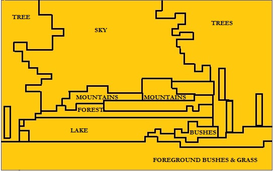
In 1969, Elwood Shafer, a researcher in the US Forest Service, published a unique approach to measuring landscape preferences by measuring areas and perimeters of features on 8” x 10” black-and-white photographs (Shafer et al, 1969). The photographs were of scenes across the US and included forests, mountains, meadows, water and various combinations. A total of 100 photographs were used. A 1/4” clear plastic grid was overlaid on each photograph, and the areas of landscape zones were then outlined by pen and measured. The 10 landscape zones were:

• sky;
• vegetation in the foreground, mid-distance and distant;
• non-vegetation (e.g. exposed ground, mountains, snowfields, grasslands) in the foreground, mid-distance and distant;
• water – streams, waterfall and lakes.

Figure 13 indicates the landscape zones identified in a scene of a lake and distant mountains, framed by trees. Each polygon is identified as a set (S_n) that identifies the total squares it contains. Each set is identified by computer, using variables that describe its boundary; the interior number of squares; the area; and the horizontal end-squares. The tonal variations provided by sky, land and water are measured by a photometer and are included in the analysis. Each photograph is described by a total of 46 variables. This was subsequently reduced to 26 zones by removing redundancies.

The photographic evaluations that describe the elements in the landscape provide the independent variables in the research method. The rating of landscape quality provides the dependent variable and was assessed by asking participants to rank the landscape on a 1 – 5 scale. Factor analysis identified nine independent factors, and the model derived used ten terms and explained 65% of the variation in landscape preference.

Using the model, the predicted scores of the 100 photographs ranged from 84 to 236 which approximated that derived from participants (Table 4).

Table 4   Shafer’s Predictive Model of Landscape Preferences

Y = 184.8 – 0.5436 X₁ – 0.0929 X₂ + 0.002069 (X₁.X₃) + 0.0005538 (X₁.X₄) – 0.002596 (X₃.X₅) + 0.001634 (X₂.X₆) – 0.008441 (X₄.X₆) – 0.0004131 (X₄.X₅) + 0.0006666 X₁² + 0.0001327 X₅²

where:     Y  = preference, X₁ = perimeter of near vegetation,  X₂ = perimeter of middle distant vegetation, X₃ = perimeter of distant vegetation, X₄ = area of near vegetation, X₅ = area of any kind of water, X₆ = area of distant non-vegetation.

Note: negative items contribute positively, while positive items contribute negatively (i.e. the lower the score the better the landscape).

Factors which had a positive influence on the landscape’s aesthetic appeal were the:

• perimeters of near and middle distant vegetation
• perimeter of distant vegetation multiplied by the area of water
• area of middle distance vegetation multiplied by the area of distant non-vegetation
• area of middle distant vegetation multiplied by the area of water.

The resultant scores are ordinal numbers that enable ranking of photographs.

Shafer has applied the method to several further studies. From an analysis, he suggested that farmland scenes could be improved by

• eliminating tree cover in the middle distance and by replacing it with fields or pasture
• establishing a lake
• permitting vegetation to encroach in the distant zone

For each of these he was able to predict the change to the score that would result (e.g. establishing a lake would improve the score from 155 to 119 – the lower is better).

Shafer’s model was criticised as “lacking intuitive appeal since some of the multiplicative independent variables, although mathematically proper, seem illogical (e.g. area of water X area of intermediate veg.)” (Buhyoff & Leuschner, 1978). Whittow (1976) suggested that the method was like the “well-known analogy of the computer attempting to describe Shakespeare,” but he also recognised its worth. The philosopher, Alan Carlson (1977), issued a lengthy critique of the method in which he identifies three key assumptions in the model:

1)       the aesthetic quality of the landscape is meaningfully correlated with certain preferences for that landscape;
2)       the relevant preferences are those of the general public;
3)       the presence of the formalist theme.

Of these, the third is possibly the most telling. Carlson notes that the methodology is “completely formalist” as the methodology measures only formal aspects of photographs – the shapes of the zones, not their contents, or the relationships between the shapes and lines. Formalism derives from the artistic tradition and identifies certain formal aspects of a scene such as shapes, lines, color, patterns, and the formal qualities which they produce such as balance, proportion, unity and diversity.

Bourassa (1991) also identified the formalist basis of Shafer’s approach and was critical of its lack of theoretical origin, stating that the “choice of variables is completely without justification (and) do not even seem to make sense intuitively.” Bourassa considered the results quite “spurious” as there is no causal link between the independent variables (i.e. the landscape’s formal qualities) and the dependent variable (i.e. preference scores). In another critique, Weinstein is also critical of Shafer’s use of regression analysis:

“With enough independent variables a regression equation can be derived that will correlate perfectly with any dependent variable, no matter how meaningless and inappropriate the predictors actually are” (Weinstein, 1976).

Despite its critics, Shafer’s approach has been used widely, simply because as it provides an objective basis for measuring the independent variable in landscape research.

Research Instruments – Conclusions

The diversity of instruments used in the evaluation of landscape preferences is notable. Although the field of landscape research is relatively new, it has been characterized by considerable innovation and imagination in the application and modification of existing techniques and the development of new ones.